Regression problems pop up whenever we want to predict a numerical value.
- Linear Model
- Loss Fuction
- Minibatch Stochastic Gradient Descent
- vectorization for speed
- The Normal Distribution and Squared Loss
- Deep network
1. Linear Model


let's say we want to predict y (label, target) through training set x.
x(i) represents ith example(sample) of the training dataset. Thoese independent variables x1(i), x2(i) are called features(covariates).

The linearity assumption just says that the label can be expressed as a weighted sum of the features.
w1, ..., wd are called weights. b is called a bias(offset, intercept).
The weights determine the influence of each feature on our prediction.
Bias just says what value the predicted price should take when all of the features take value 0.
Out goal is to choose the w and b to make our model best fit the true label.


let's say there are d features, if we use linear algebra notation. It can be expressed like equation below

In this equation vector x corresponds to features of a single data example.

it is more convenient to refer to features of our entire dataset of n examples.
one row for every example and one column for every features.


2. Loss Functions
Loss function is a measure of fitness. How far from real to predicted value of the target.
squared error is the most populate loss function in regression problems.


1/2 makes no real difference but it is way convenient, canceling out when we take derivative of the loss.

To measure the quality of a model on the entire dataset of n examples, we simply average (or equivalently, sum) the losses on the training set.

Again our goal is to find parameters (w*, b*) that minimize the total loss across all training examples.
3. Minibatch Stochastic Gradient Descent
The key technique of optimizing is iteratively reducing the error by updating the parameters in the direction that incrementally lowers the loss function. (Gradient descent)
Gradient descent consists of taking the derivative of the loss function, which is an average of the losses computed on every single example in the dataset. But it is extremely slow: pass the eintire dataset before making a signle update.
Thus, we will often settle for sampling a random minibatch of examples every time we need to compute the update, a variant called minibatch stochastic gradient descent.

Compute the derivative (gradient) of the average loss on the minibatch with regard to the model parameters.
The cardinality |B| represents the number of examples in each minibatch (the batch size) and η denotes the learning rate. These parameters that are tun- able but not updated in the training loop are called hyperparameters.
Our final goal is not finding minima of loss on training set but find parameters that will achieve low loss on data that we have not seen before, a challenge called generalization.
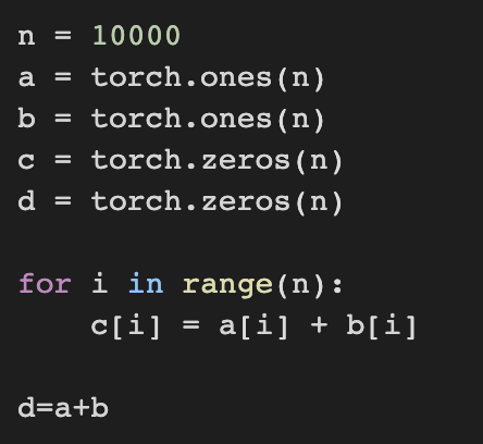
4. Vectorization for speed
vectorize the calculations and leverage fast linear algebra libraries rather than writing costly for-loops in Python.

5. The Normal Distribution and Squared Loss
https://angeloyeo.github.io/2020/07/17/MLE.html
최대우도법(MLE) - 공돌이의 수학정리노트
angeloyeo.github.io
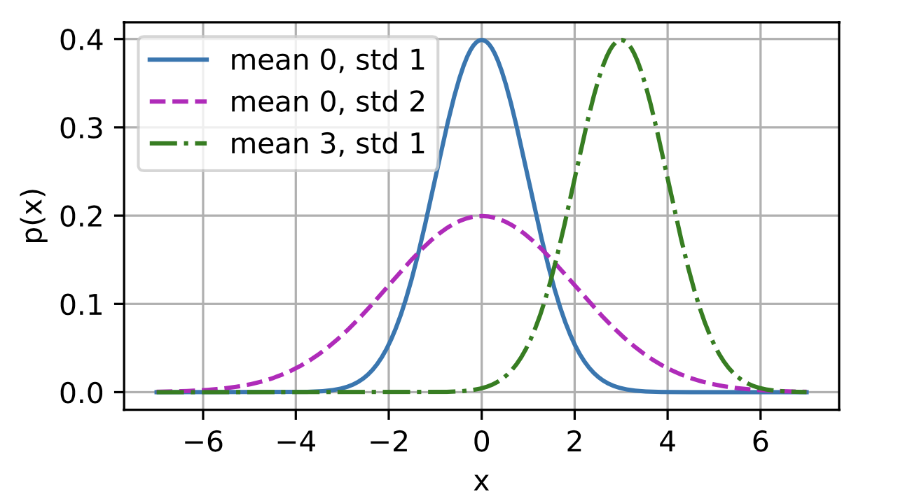
normal distribution is also called Gausian

mean μ and variance σ^2

One way to motivate linear regression (with the mean squared error loss function ) is to formally assume that observations arise from noisy observations, where the noise is normally distributed as follows:

likelihood of seeing a particular y for a given x via (가능도)

according to the principle of maximum likelihood, the best values of parameters w and b are those that maximize the likelihood of the entire dataset

Now we have to find w, b which maximize the likelihood but instead minimize the negative log-likelihood − log P (y | X).

if we that σ is some fixed constant. the first term and sigma of second term can be ignored.
It follows that minimizing the mean squared error is equivalent to maximum likelihood estimation of a linear model under the assumption of additive Gaussian noise.
6. Deep network
let's depict our linear regression model as a neural network
Note that these diagrams are just for highlighting the connectivity pattern of input and output

inputs are x1, . . . , xd, so the number of inputs (or feature dimensionality) in the input layer is d.
conventionally we do not consider the input layer when counting layers. So the number of layers for the nueral network is 1 (single-layer neural networks)
Since for linear regression, every input is connected to every output (in this case there is only one output), we can regard this transformation (the output layer in Fig. 3.1.2) as a fully-connected layer or dense layer.
'ComputerScience > Machine Learning' 카테고리의 다른 글
| Deep Learning - 2.3 Concise Implementation of Linear Regression (0) | 2022.08.16 |
|---|---|
| Deep Learning - 2.2 Linear Regression Implementation from Scratch (0) | 2022.08.13 |
| Deep Learning - 1.6 Probability (0) | 2022.08.09 |
| Deep Learning - 1.5 Automatic Differentiation (0) | 2022.08.06 |
| Deep Learning - 1.4 Calculus (0) | 2022.08.03 |


