How do we get solutions x from a system of linear equations, Ax = b.
If we have a particular solution x_p such that Ax_p = B, and a homogenous solution x_h such that Ax_h = 0, then any scalar t.
A(x_p + t*x_h) = b
x = x_p + t*x_h
Thus, adding any multiple of a homogeneous solution to a particular solution still satisfies the original solution.
Notice that neither the general nor the particular solution is unique.
Let's say we have a system of linear equations.

1. Find a Particular Solution
1.1 Convert to Row Echelon Form(REF)
-2   4  -2  -1  4 | -3
 4  -8   3  -3  1 |  2
 1  -2   1  -1  1 |  0
 1  -2   0  -3  4 |  a

 ---------------------- change R1, R3

  1  -2   1  -1  1 |  0
 -2   4  -2  -1  4 | -3
  4  -8   3  -3  1 |  2
  1  -2   0  -3  4 |  a

---------------------- R2 <-R2 + 2R1

  1  -2   1  -1  1 |  0
  0   0   0  -3  6 | -3
  4  -8   3  -3  1 |  2
  1  -2   0  -3  4 |  a

 ---------------------- R3 <-R3 - 4R1

  1  -2   1  -1  1 |  0
  0   0   0  -3  6 | -3
  0   0  -1   1 -3 |  2
  1  -2   0  -3  4 |  a

 ---------------------- R4 <-R4 - R1

  1  -2   1  -1  1 |  0
  0   0   0  -3  6 | -3
  0   0  -1   1 -3 |  2
  0   0  -1  -2  3 |  a

 ---------------------- R4 <-R4 - R3

  1  -2   1  -1  1 |  0
  0   0   0  -3  6 | -3
  0   0  -1   1 -3 |  2
  0   0   0  -3  6 |  a-2

 ---------------------- R4 <-R4 - R2

  1  -2   1  -1  1 |  0
  0   0   0  -3  6 | -3
  0   0  -1   1 -3 |  2
  0   0   0   0  0 |  a+1

  ----------------------change R2, R3

  1  -2   1  -1  1 |  0
  0   0  -1   1 -3 |  2
  0   0   0  -3  6 | -3
  0   0   0   0  0 |  a+1

  ---------------------- R2 <- -R2 and R3 <- R3/(-3)

  1  -2   1  -1  1 |  0
  0   0   1  -1  3 | -2
  0   0   0   1 -2 |  1
  0   0   0   0  0 |  a+1
1.2. Particular Solution
So the the final echelon form is (the echelon form is not unique)
  1  -2   1  -1  1 |  0
  0   0   1  -1  3 | -2
  0   0   0   1 -2 |  1
  0   0   0   0  0 |  a+1
 x1  x2  x3  x4 x5
basic variable, pivot : x1, x3, x4
free variable : x2, x5
and a should be -1
Simpy we can get a particular solution x_p, which is obviously not unique
- 1. R3 : 1x4 -2x5 = 1, set x5 = 0 and let x4 =1
- x_p = [?, ?, ?, 1, 0]
- 2. R2 : 1x3 -1x4 + 3x5 = -2 -> 1x3 - 1(1) + 3(0) = -2 -> 1x3 -1 = -2
- x_p = [?, ?, -1, 1, 0]
- 3. R1 : 1x1 -2x2 + 1x3 -1x4 + 1x5 = 0 -> 1x1 -2x2 + 1(-1) -1(1) + 1(0) = 0 -> 1x1 -2x2-2 = 0 , let x2=0
- x_p = [2, 0, -1, 1, 0]
2. Find a solution of homogenous solution
2.1. Convert to Reduced Row Echelon Form (RREF)
  1  -2   1  -1  1 |  0
  0   0   1  -1  3 |  0
  0   0   0   1 -2 |  0
  0   0   0   0  0 |  0

------------------------- R1 <- R1 - R2

  1  -2   0   0 -2 |  0
  0   0   1  -1  3 |  0
  0   0   0   1 -2 |  0
  0   0   0   0  0 |  0

------------------------- R2 <- R2 + R3

  1  -2   0   0 -2 |  0
  0   0   1   0  1 |  0
  0   0   0   1 -2 |  0
  0   0   0   0  0 |  0
 x1  x2  x3  x4 x5
2.2 Homogenous Solution
RREF makes finding the solution quite straightforward, the key idea is to express non-pivot columns as a linear combination of the pivot columns that are on their left.
R3 : x4 = (2) * x5
R2 : x3 = (-1) * x5
R1 : x1 = (2) * x5 + (2) * x2

2.2.1 Minus-1 Trick
  1  -2   0   0 -2 |  0
  0   0   1   0  1 |  0
  0   0   0   1 -2 |  0
  0   0   0   0  0 |  0

 --------------------- insert rows [...-1...] at the places where the pivots are missing

  1  -2   0   0 -2 |  0
  0  -1   0   0  0 |  0
  0   0   1   0  1 |  0
  0   0   0   1 -2 |  0
  0   0   0   0 -1 |  0
By taking the columns of the new A which contain -1 on the diagonal, we can immediately read out the solutions of Ax=0
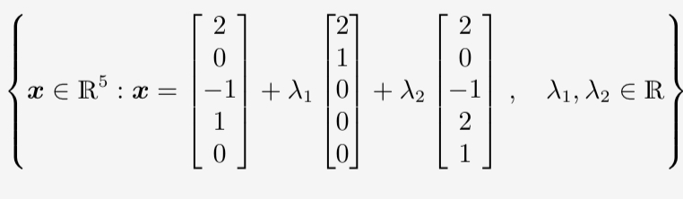
3. General Solution
particular solution : x_p = [2, 0, -1, 1, 0]
homogenous solution : (above)
So the general solution x = x_p + t*x_h
Appendix. Calculating the Inverse
To comput the inverse A^-1 of A ∈ R^n*n, we need to find X that satisfies AX = I_n.
[A | I_n] -> ... -> [I_n | A^-1]
A =
1 0 2 0
1 1 0 0
1 2 0 1
1 1 1 1
------------- write down augmented matrix
1 0 2 0 | 1 0 0 0
1 1 0 0 | 0 1 0 0
1 2 0 1 | 0 0 1 0
1 1 1 1 | 0 0 0 1
------------- transform into RREF
1 0 0 0 |-1  2 -2  2
0 1 0 0 | 1 -1  2 -2
0 0 1 0 | 1 -1  1 -1
0 0 0 1 |-1  0 -1  2
-------------
A^-1 =
-1  2 -2  2
 1 -1  2 -2
 1 -1  1 -1
-1  0 -1  2
In special cases, we may be able to determine the inverse A^-1, such that the solution of Ax=b is given as x = A^-1*b.
However, this is only possible if A is a square matrix and invertible.
Otherwise, under mild assumption we can use the transformation.
Ax=b -> A.T * A = A.T * b -> x = (A.T * A)^-1 * A.T * b
and use the Moore-Penrose pseudo-inverse (A.T * A)^-1 * A.T to determine the solution
'boostcamp AI tech > boostcamp AI' 카테고리의 다른 글
| [Math] Linear Independent, Span, Basis and Rank (1) | 2024.10.10 |
|---|---|
| [Math] Groups, Vector Spaces and Vector Subspaces (0) | 2024.10.02 |
| [PyTorch] Modify Gradient while Backward Propagation Using Hook (0) | 2024.09.27 |
| [Math] Viewing Deep Learning From Maximum Likelihood Estimation Perspective (0) | 2024.09.25 |
| Docker (1) | 2024.03.06 |


