We can see finding deep learning model's parameters from maximum likelihood estimation perspective.
1. Normal distribution
1.1 Setting
Let's say we have a model μ = wx+b
and have a dataset {(x₁, y₁), ..., (x₁, y₅), (x₂, y₆), ... , (x₂, y₁₁), (x₃, y₁₂), ...} consists of n samples.
1.2 Assume a probability distribution

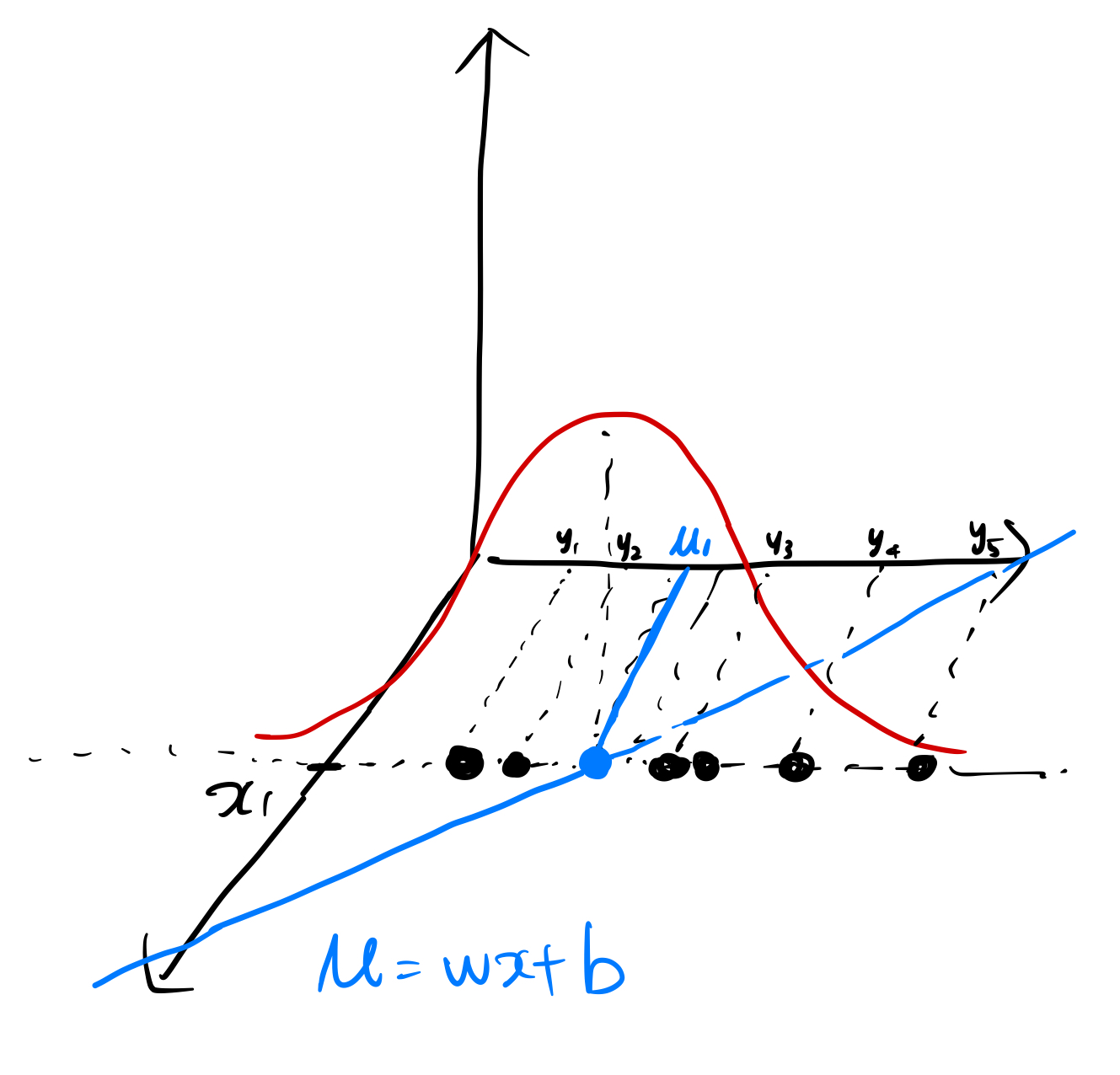
Let's assume the observed value y, given x, follows normal distribution with mean μ=wx+b and some variance σ².
y ~ N(wx + b, σ²)
Then we can define PDF(y) = p(y|x) = (1 / √(2πσ²)) * exp(-(y - (wx + b))² / (2σ²)).
p(y) is an equation with given x, so p(y) can be denoted as p(y|x).
1.3 Write Likelihood function
Likelihood is a joint probability of observing the given data, given a specific set of parameter values.
Given n independent data points {(x₁, y₁), ..., (x₁, y₅), (x₂, y₆), ... , (x₂, y₁₁), (x₃, y₁₂), ...}, the likelihood function becomes,
L(θ | {(x₁, y₁), ..., (x₁, y₅), (x₂, y₆), ... , (x₂, y₁₁), (x₃, y₁₂), ...})
= p({(x₁, y₁), ..., (x₁, y₅), (x₂, y₆), ... , (x₂, y₁₁), (x₃, y₁₂), ...} | θ)
= p(y₁ | x₁ ; θ) * ... * p(yₙ | xₙ ; θ)
So getting back to our case,
L(w, b, σ² | x, y)
= Π[i=1 to n] p(y_i | x_i; w, b, σ²)
= Π[i=1 to n] (1 / √(2πσ²)) * exp(-(y_i - (wx_i + b))² / (2σ²))
1.4. Take the log of the likelihood to simplify calculation (log-likelihood)
ln L(w, b, σ² | x, y) = Σ[i=1 to n] [-ln(√(2πσ²)) - (y_i - (wx_i + b))² / (2σ²)]
1.5 Optimization
Calculate the gradients of the negative log-likelihood with respect to w and b.
Update w and b using these gradients.
1.6 Connect to common loss functions
maximize the log-likelihood
= minimizing the negative log-likelihood
= minimizing sum of squared errors (y_i - (wx_i + b))²
which is why MSE loss function is commonly used in deep learning regression problems.
1.7 Interpretation
By minimizing the negative log-likelihood (or MSE loss), we're finding the parameters w and b that make our observed data most probable under our model assumptions.
The choice of loss function often implies an assumption about the distribution of the model's output, which means when using, for example, MSE, we are assuming model's ouput would follow normal distribution.
So we can say, after training, what kind of distribution the model's output will have depends on what kind of loss we are using.
Choosing an appropriate loss function is not just about minimizing an arbitrary error metric, but about making a statistical assumption about the problem we're modeling.
2. Bernoulli distribution
2.1 Setting
Let's say we have a model, y = σ(w₁x₁ + w₂x₂ + b), where σ is the sigmoid function
and dataset, {(x₁₁, x₁₂, y₁), (x₂₁, x₂₂, y₂), (x₃₁, x₃₂, y₃)}
2.2 Assume probability distribution
k ~ Bernoulli(σ(w₁x₁ + w₂x₂ + b))
p(k|x) = σ(w₁x₁ + w₂x₂ + b)^k * (1 - σ(w₁x₁ + w₂x₂ + b))^(1-k), where the probability of k=1 is given by σ(w₁x₁ + w₂x₂ + b).
2.3 Write Likelihood function
L(w₁, w₂, b | X, Y) = Π[i=1 to 3] P(yᵢ|xᵢ₁, xᵢ₂) = Π[i=1 to 3] [σ(w₁xᵢ₁ + w₂xᵢ₂ + b)^yᵢ * (1 - σ(w₁xᵢ₁ + w₂xᵢ₂ + b))^(1-yᵢ)]
2.4. Take the log of the likelihood to simplify calculation (log-likelihood)
ln L(w₁, w₂, b | X, Y) = Σ[i=1 to 3] [yᵢ ln(σ(w₁xᵢ₁ + w₂xᵢ₂ + b)) + (1-yᵢ) ln(1 - σ(w₁xᵢ₁ + w₂xᵢ₂ + b))]
2.5 Connect to common loss function
This is exactly the Binary Cross-Entropy Loss = -Σ[i=1 to N] [yᵢ log(pᵢ) + (1-yᵢ) log(1-pᵢ)]
3. Categorical Distribution
3.1 Setting
π = softmax(z)
z = W₂ * σ(W₁x + b₁) + b₂
x is the input vector
- W₁ and b₁ are the weight matrix and bias vector for the hidden layer
- W₂ and b₂ are the weight matrix and bias vector for the output layer
- σ is an activation function (e.g., ReLU)
Specifically:
- π₁ = exp(z₁) / (exp(z₁) + exp(z₂) + exp(z₃))
- π₂ = exp(z₂) / (exp(z₁) + exp(z₂) + exp(z₃))
- π₃ = exp(z₃) / (exp(z₁) + exp(z₂) + exp(z₃))
Here, π₁, π₂, and π₃ represent the probabilities of the input belonging to class 1, 2, and 3 respectively.
And suppose we have N data points: {(x₁, y₁), (x₂, y₂), ..., (xₙ, yₙ)} where each yᵢ is a one-hot encoded vector representing the true class.
3.2 Assume Probability Distribution
k ~ Categorical(π₁, π₂, π₃)
p(k|x; θ) = π₁^y₁ * π₂^y₂ * π₃^y₃, where π₁ + π₂ + π₃ = 1
3.3 Write Likelihood function
L(θ|X,Y) = Π[i=1 to N] (π₁ᵢ^y₁ᵢ * π₂ᵢ^y₂ᵢ * π₃ᵢ^y₃ᵢ)
3.4. Take the log of the likelihood to simplify calculation (log-likelihood)
ln L(θ|X,Y) = Σ[i=1 to N] (y₁ᵢln(π₁ᵢ) + y₂ᵢln(π₂ᵢ) + y₃ᵢln(π₃ᵢ))
3.5 Connect to common loss function
This is exactly the Categorical Cross-Entropy Loss = -Σ[i=1 to N] Σ[j=1 to k] yᵢⱼ log(pᵢⱼ)
'boostcamp AI tech > boostcamp AI' 카테고리의 다른 글
| [Math] Finding Solutions of a System of Linear Equations (0) | 2024.09.28 |
|---|---|
| [PyTorch] Modify Gradient while Backward Propagation Using Hook (0) | 2024.09.27 |
| Docker (1) | 2024.03.06 |
| Airflow (0) | 2024.02.26 |
| Product Serving 관련 용어 정리 (0) | 2024.02.26 |


