[Paper Review] Sequence Transduction with Recurrent Neural Networks

 

Sequence Transduction with Recurrent Neural Networks

---

0. Abstract

Many machine learning tasks can be expressed as the transformation—or transduction —of input sequences into output sequences: speech recognition, machine translation and so on
One of the key challenges in sequence transduction is learning to represent both the input and output sequences in a way that is invariant to sequential distortions such as shrinking, stretching and translating.

• Normal: "Hello, how are you?" 
• Different Voices: "Hello, how are you?" 
• Shrinking: "H'llo, how're you?" (faster speech) 
• Stretching: "Heeeello, hoooow aaaare yooou?" (slower speech) 
• Translating: "...Hello, how are you?" (delayed start)

RNNs traditionally require a pre-defined alignment between the input and output sequences to perform transduction. This is a severe limitation since finding the alignment is the most difficult aspect of many sequence transduction problems.

• The model needs to know which parts of the input correspond to which parts of the output.
• The alignment between audio segments and corresponding words is not straightforward. Speakers may pause, stretch words, or speak at different speeds.

This paper introduces an end-to-end, probabilistic sequence transduction system, based entirely on RNNs, that is in principle able to transform any input sequence into any finite, discrete output sequence

1. Introduction

(Traditional) RNNs are usually restricted to problems where the alignment between the input and output sequence is known in advance.

• Input: Audio frames of a speech signal
• Output: Classification for each frame (e.g., phoneme or silence)
• Alignment: One-to-one correspondence between input frames and output classifications
• If the network outputs are probabilistic this leads to a distribution over output sequences of the same length as the input sequence. But for a general-purpose sequence transducer, where the output length is unknown in advance, we prefer distribution over sequences of all length

Connectionist Temporal Classification (CTC) is an RNN output layer that defines a distribution over all alignments with all output sequences not longer than the input sequence

• such as text-to-speech, where the output sequence is longer than the input sequence, CTC does not model the interdependencies between the outputs.

CTC assumes conditional independence between output tokens, which means it doesn't model how one output element might influence the next.

The transducer described in this paper extends CTC by defining a distribution over output sequences of all lengths, and by jointly modelling both input-output and output-output dependencies.

• Distribution Over All Lengths: The advanced transducer can generate output sequences of any length, not constrained by the input length.
• Modeling Dependencies: It captures both input-output and output-output dependencies, leading to more coherent and contextually appropriate outputs.

2. Recurrent Neural Network Transducer

Sequence-to-sequence learning with Transducers

Transducer defines p(y|x) as sum of the probabilities of all possible alignments between x and y.

• x : (x_1,x_2,...,x_T), input sequence of length T
  • If the task is phonetic speech recognition, each x_t would typically be a vector of MFC coefficients
• X^* : all input sequences of arbitrary length
• y : (y_1, y_2, . . . , y_U) output sequence of length U
  • each y_t would be a one-hot vector encoding a particular phoneme.
• Y^* : all output sequences of arbitrary length
  • (y_1, y_2, y_3) ∈ Y^* 
• Y- : extended output space
  • Y U '_' 
  • (y_1, _ , _ , y_2, _ , y_3) ∈ (Y-)^* 
  • refer to the element a ∈ (Y-)^* as alignments
• B : (Y-)^∗ → Y^∗, removes the null symbols from the alignments in (Y-)^∗

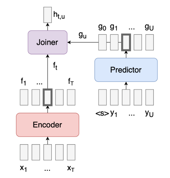
Two recurrent neural networks are used to determine Pr(y | x)

• Transcription network F (Encoder)
  • x -> f = (f_1, ... , f_T)
  • Encodes the input sequence, capturing its important features and contextual information
  • f_i is a vector of the number of labels, K + 1
• Prediction network g (Predictor)
  • y = (_, y_1, ..., y_U) -> g = (g_0, g_1, ..., g_U)
  • Decodes the output sequence y
  • y_i is a vector of the number of labels, K
  • g_i is a vector of the number of labels, K + 1
  • language model is used to inject prior knowledge about the output sequences, it must also be robust to missing words, mis- pronunciations, non-lexical utterances etc

2.1 Prediction Network

Prediction network g is a recurrent neural network consisting of an input layer, an output layer and a single hidden layer.

• input
  • y^ = ( _ , y_1, ... , y_U) 
  • length U+1 input, _ is prepended to input sequence y
  • y_i is encoded as one-hot vectors of K labels, all zeros except ith position which is one.
  • _ token is encoded as a vector of K zeros.
    • y = "ab" -> yˆ = (∅, a, b) -> [[0,0,0], [1,0,0], [0,1,0]]
• output 
  • g = (g_0, g_1, ... , g_U)
  • K+1 size which include _, null token

Given y^, g computes the hidden vector sequence (h0,...,hU) and the prediction sequence (g0,...,gU) by iterating the following equations from u = 0 to U

 

The prediction network attempts to model each element of y given the previous ones; it is therefore similar to a standard next-step-prediction RNN, only with the added option of making ‘null’ predictions. (capture output-output dependencies)

 

2.2 Transcription Network

Transcription network F is a bidirectional RNN that scans input sequence x.

• input : x = (x_1, ..., x_T)
• forward hidden : (h_1, ..., h_T)
• backward hidden : (h_1, ..., h_T)
• output : f = (f_1, ..., f_T) 
  • f_i is a vector of the number of labels, K + 1

The transcription network is similar to a Connectionist Temporal Classification RNN, which also uses a null output to define a distribution over input-output alignments.

 

2.3 Output Distribution

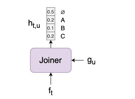
With f_t, g_u, k, we can define the output density function

• k : possible output label k ∈ Y- (a ∈ {_ , a, b, c})
  • superscript k : k-th element of the vector f_t/g_u
  • ex) f_t에서 phoneme k일 확률, g_u에서 phoneme k일 확률로 t, u 시점에서 phoneme k일 확률을 구한다.
• f_t : transcription vector  (1 ≤ t ≤ T)
• g_u : prediction vector (0 ≤ u ≤ U)

 

The density can be normalised to yield the conditional output distribution (f_t와 g_u를 더한 값을 softmax에 통과시키는 것과 동일)

• Let's say we have a simple case with only three possible labels: Ȳ = {A, B, C}. Assume we're at time step t=3 in the input and u=2 in the output. 
  • Step 1: Calculate h(k,t,u) for each label: 
    • Suppose we get these values: 
    • h(A,3,2) = exp(2.5) ≈ 12.18 
    • h(B,3,2) = exp(1.8) ≈ 6.05 
    • h(C,3,2) = exp(0.9) ≈ 2.46 
  • Step 2: Calculate the sum of all h(k,t,u): 
    • ∑k'∈Ȳ h(k',3,2) = 12.18 + 6.05 + 2.46 = 20.69 
  • Step 3: Normalize to get probabilities: 
    • Pr(A|3,2) = 12.18 / 20.69 ≈ 0.589 
    • Pr(B|3,2) = 6.05 / 20.69 ≈ 0.292 
    • Pr(C|3,2) = 2.46 / 20.69 ≈ 0.119
  • Now we have a proper probability distribution: The probabilities are non-negative.
  • They sum to 1 (0.589 + 0.292 + 0.119 = 1). 

simplified notation.

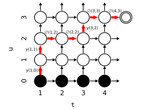
The set of possible paths from the bottom left to the terminal node in the top right corresponds to the complete set of alignments between x and y

• Pr(y_(u+1)|t,u)는 다음 phoneme, y_(u+1)을 예측할 확률 
• Pr(∅|t,u)는 다음에 ∅일 확률이다.

2.4 Forwad-Backward Algorithm

• a(t,u) : forward variable, the probability of outputting y_[1:u] during f_[1:t]
• a(1,0) : 1, always starts from bottom left node.

The total output sequence probability is equal to the forward variable at the terminal node,

 

• β(t,u) : backward variable, the probability of outputting y_[u+1,U] during f_[t:T]

product α(t, u)β(t, u) at any point (t,u) in the output lattice is equal to the probability of emitting the complete output sequence if y_u is emitted during transcription step t.

• t시점에 u를 뱉었을 경우 output sequence가 가능한 모든 경로들의 확률의 합

 

2.5 Training

• y* : target sequence, all possible alignments
• x : input

• equal to the sum of α(t,u)β(t,u) over any top-left to bottom-right diagonal through the nodes
• ∀n:1≤n≤U+T

각 노드가 가리키는 확률을 α(t, u)β(t, u)라고 하면, 파랑박스 속 노드들의 확률합이 Pr(y*|x)이다.

모든 n에 대해 가능하다는 말은 얘도 가능하다는 뜻이다. 두 파랑 박스의 확률은 같다. initial point에서 terminal point로 전이되는 모든 확률은 대각선을 뚫고 가야 하기 때문에 top-left, bottom-right의 대각선의 확률합이 Pr(y*|x)인 것이다.

다만 Pr(k|t,u)에 대해서 미분하기 편하게 하기 위해 top-left, bottom-right의 대각선을 사용한다.

정말 명확한 식이다. 이해가 안된다면 잘~생각해보자

13은 소프트맥스의 미분이다

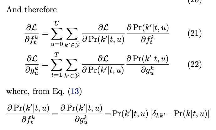
• δkk' : Kronecker delta (1 if k=k', 0 otherwise).
• δL/δf_tk = δL/δf(k|t,0) + δL/δf(k|t,1) +  ... + δL/δf(k|t,U)

2.5.1 Optimization technique for computing the conditional probabilities

• Naive Approach
  • Initially, one might compute a separate softmax for each Pr(k|t,u) required by the forward-backward algorithm. This would involve calculating exp(ftk + guk) for each combination of t, u, and k.
• Problem with Naive Approach:
  • This is computationally expensive because:
  • The exponential function is costly to compute.
  • There are many combinations of t, u, and k, leading to O(TU) exponential evaluations.
• Optimization Using Exponential Properties:
  • The key insight is using the property: exp(a + b) = exp(a) * exp(b)
• Optimized Approach:
  • Precompute exp(ftk) for all t and k
  • Precompute exp(guk) for all u and k
  • Use these precomputed values to calculate h(k,t,u) = exp(ftk) * exp(guk)
• Benefit:
  This reduces the number of exponential evaluations from O(TU) to O(T + U)
  Let's illustrate this with an example:
• Assume we have:
  • Input sequence length T = 100
  • Output sequence length U = 50
  • Number of labels |Ȳ| = 10
• Naive Approach:
  • Number of exp evaluations = T * U * |Ȳ| = 100 * 50 * 10 = 50,000
• Optimized Approach:
  • exp evaluations for input: T * |Ȳ| = 100 * 10 = 1,000
  • exp evaluations for output: U * |Ȳ| = 50 * 10 = 500
  • Total exp evaluations = 1,000 + 500 = 1,500

3. Experimental Results

PREDICTION is the standalone prediction network of TRANSDUCER

TIMIT transcriptions are too small a training set for the prediction network : as opposed to the millions of words typically used to train language models
This is supported by the poor performance of the standalone prediction network
Alternatively the prediction network could be pretrained on a large ‘target-only’ dataset, then jointly retrained on the smaller dataset as part of the transducer.

Figure 3.  Visualisation of the transducer applied to end-to-end speech recognition

• the heat map in the top right
  • shows the log-probability of the target sequence passing through each point in the output lattice.
• The image immediately below heatmap
  • shows the input sequence (a speech spectrogram),
• The image immediately to the left heatmap
  • shows the inputs to the prediction network (a series of one-hot binary vectors encoding the target characters).

Note the learned ‘time warping(전이, 경로)’ between the two sequences(input and output of prediction network).

Also note the blue ‘tendrils’, corresponding to low probability alignments,

short vertical segments, corresponding to common character sequences (such as ‘TH’ and ‘HER’) emitted during a single input time step. (한 시점에서 여러 character 출력)

 

• The bar graphs in the bottom left
  • indicate the labels most strongly predicted by the output distribution (blue), the transcription function (red) and the prediction function (green) at the point in the output lattice indicated by the crosshair(하얀 가로세로 분할 선의 교착 지점).
  • In this case the transcription network simultaneously predicts the letters ‘O’, ‘U’ and ‘L’, presumably because these correspond to the vowel sound in ‘SHOULD’; the prediction network strongly predicts ‘O’; and the output distribution sums the two to give highest probability to ‘O’.
• The heat map below the input sequence
  • shows the sensitivity of the probability at the crosshair to the pixels in the input sequence
  • the transcription network is more sensitive to parts of the spectrogram with higher energy.
  • The sensitivity of the transcription network extends in both directions because it is bidirectional, unlike the prediction network.

• the heat map to the left of the prediction inputs
  • shows the sensitivity of the the probability at the crosshair to the previous outputs.
  • the dark horizontal bands in the prediction heat map; these correspond to a lowered sensitivity to spaces between words.

These maps suggest that both networks are sensitive to long range dependencies, with visible effects extending across the length of input and output sequences.

 

4. Decoding

Consider an input sequence of length T=4 and an output sequence ("CAT") of length U=3

one alignment:  z=∅,C,A,∅,T,∅,∅ and another z = C , ∅ , A , ∅ , T , ∅ , ∅

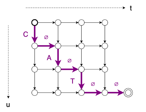
1. Start by setting t:=1, u:=0, and y:= an empty list.
2. Compute f_t using x and g_u using y.
3. Compute h_t,u using f_t and g_u.
   1. If the argmax of h_t,u is a label, set u:=u+1, and output the label (append it to y and feed it back into the predictor).
   2. If the argmax of h_t,u is ∅, set t:=t+1 (in other words, just move to the next input timestep and output nothing).
4. If t=T+1, we’re done. Else, go back to step 2.

 

5. Appendix - Training vs Decoding

There's an important distinction between the training (forward pass) and decoding processes in RNN Transducer models. Let's break this down:

1. Forward Pass (Training):
During training, the forward function typically processes entire sequences at once. The outputs of the encoder and prediction network are indeed concatenated or combined in some way for all time steps and all possible output tokens. This is done to compute the full output distribution efficiently for the loss calculation.

The shape of the encoder output is usually (batch_size, input_length, encoder_dim), while the prediction network output is (batch_size, target_length, prediction_dim). These are combined in the joint network to produce an output of shape (batch_size, input_length, target_length, joint_dim).

2. Decoding (Inference):
During decoding, the process is sequential and depends on whether the predicted token is blank or not:
- If blank is predicted, we move to the next encoder time step without updating the prediction network state.
- If a non-blank token is predicted, we feed this token back into the prediction network and stay at the same encoder time step.

This sequential process isn't reflected in the forward function because it's specific to the decoding algorithm, not the training process.

3. Why the difference?
- Training: We need to compute probabilities for all possible alignments to calculate the loss efficiently. This is why we process all combinations of encoder and prediction network outputs.
- Decoding: We generate one token at a time, making decisions based on each output, which is why we see the blank/non-blank logic.

4. Shape Consistency:
While the shapes of the encoder and prediction network outputs are different, they are made compatible in the joint network. This is typically done by broadcasting or repeating the outputs to match dimensions before combining them.

For example, if we have:
- Encoder output: (batch_size, input_length, encoder_dim)
- Prediction output: (batch_size, target_length, prediction_dim)

The joint network might do something like:

encoder_output = encoder_output.unsqueeze(2).expand(-1, -1, target_length, -1)
prediction_output = prediction_output.unsqueeze(1).expand(-1, input_length, -1, -1)
joint_output = self.joint_network(torch.cat([encoder_output, prediction_output], dim=-1))

// Initial shapes
// encoder_output: (batch_size, input_length, encoder_dim)
// prediction_output: (batch_size, target_length, prediction_dim)

// After unsqueeze
// encoder_output: (batch_size, input_length, 1, encoder_dim)
// prediction_output: (batch_size, 1, target_length, prediction_dim)

// After Expand
// encoder_output: (batch_size, input_length, target_length, encoder_dim)
// prediction_output: (batch_size, input_length, target_length, prediction_dim)

// After concatenation
// joint_input: (batch_size, input_length, target_length, encoder_dim + prediction_dim)

// After joint network
// joint_output: (batch_size, input_length, target_length, joint_dim)

This creates a 4D tensor where every combination of encoder and prediction outputs is processed.

In summary, the forward function computes the full output distribution for training, while the decoding process uses this distribution sequentially to generate predictions. The blank/non-blank logic is part of the decoding algorithm, not the forward pass.

 

5. Simple Implementation

import torch
import torch.nn as nn
import torch.nn.functional as F

class Encoder(nn.Module):
    def __init__(self, input_dim, hidden_dim):
        super().__init__()
        self.lstm = nn.LSTM(input_dim, hidden_dim, num_layers=2, bidirectional=True, batch_first=True)
    
    def forward(self, x):
        return self.lstm(x)[0]

class PredictionNetwork(nn.Module):
    def __init__(self, vocab_size, embed_dim, hidden_dim):
        super().__init__()
        self.embedding = nn.Embedding(vocab_size, embed_dim)
        self.lstm = nn.LSTM(embed_dim, hidden_dim, batch_first=True)
    
    def forward(self, x, hidden=None):
        x = self.embedding(x)
        return self.lstm(x, hidden)

class JointNetwork(nn.Module):
    def __init__(self, encoder_dim, pred_dim, output_dim):
        super().__init__()
        self.fc = nn.Linear(encoder_dim + pred_dim, output_dim)
    
    def forward(self, enc_out, pred_out):
        return self.fc(torch.cat([enc_out, pred_out], dim=-1))

class RNNTransducer(nn.Module):
    def __init__(self, input_dim, vocab_size, encoder_dim, pred_dim, embed_dim, joint_dim):
        super().__init__()
        self.encoder = Encoder(input_dim, encoder_dim // 2)
        self.prediction = PredictionNetwork(vocab_size, embed_dim, pred_dim)
        self.joint = JointNetwork(encoder_dim, pred_dim, joint_dim)
        self.fc_out = nn.Linear(joint_dim, vocab_size)
    
    def forward(self, x, y=None):
        encoder_out = self.encoder(x)
        if y is not None:
            pred_out = self.prediction(y)[0]
            joint_out = self.joint(encoder_out.unsqueeze(2), pred_out.unsqueeze(1))
            return self.fc_out(joint_out)
        return encoder_out

def greedy_decode(model, feature, max_length=100):
    encoder_out = model.encoder(feature)
    T = encoder_out.size(1)
    
    predictions = []
    t, u = 0, 0
    pred_input = torch.LongTensor([[0]])  # Start token
    pred_hidden = None

    while t < T and u < max_length:
        pred_out, pred_hidden = model.prediction(pred_input, pred_hidden)
        joint_out = model.joint(encoder_out[:, t:t+1], pred_out)
        out_probs = F.softmax(model.fc_out(joint_out).squeeze(), dim=-1)
        
        pred_token = out_probs.argmax().item()
        
        if pred_token == 0:  # blank token
            t += 1
        else:
            predictions.append(pred_token)
            pred_input = torch.LongTensor([[pred_token]])
            u += 1
        
        if t == T:
            break

    return predictions

# Example usage
input_dim = 1
vocab_size = 28  # 26 letters + blank + EOS
encoder_dim = 256
pred_dim = 128
embed_dim = 64
joint_dim = 256

model = RNNTransducer(input_dim, vocab_size, encoder_dim, pred_dim, embed_dim, joint_dim)

# Dummy input (replace with your actual feature)
feature = torch.randn(1, 1000, 1)  # [batch_size, time_steps, input_dim]

# Decode
output_indices = greedy_decode(model, feature)

# Convert indices to characters (assuming a simple mapping where 1='a', 2='b', etc.)
output_string = ''.join([chr(i + 96) for i in output_indices if i > 0])
print(f"Predicted output: {output_string}")

 

6. Appendix - CTC vs RNN-T

	RNN+ CTC	RNN Transducer
Model Architecture	encoder	encoder, predictor, joint network
Output Independence	assume output labels are independent	predictor and joint network are conditionally dependent on previous output
Language Modeling	require external LM	incorporates predictor network internally
Training	simple, easy	joint training of multiple components
Pros	- Simpler architecture and easier to train - Can work well with external language models	- Generally more accurate than CTC, even with fewer parameters - Faster convergence during training - Better handling of proper nouns and rare words - Incorporates language modeling internally, reducing the need for external language models - Can operate in online streaming mode
Cons	- Slower convergence during training - Less accurate, especially for proper nouns and rare words - Requires an external language model for optimal performance - Assumes conditional independence between outputs, leading to potential linguistic errors	- More complex architecture and training process - May require more computational resources due to multiple components
	input sequence의 길이가 반드시 output sequence보다 길다.	동일한 시간 t에서 수직 이동 경로가 가능하다. 즉 한 프레임에서도 여러개의 label이 나올 수 있다. 즉 output길이가 input sequence길이보다 길 수 있다.